After setting the record for the hottest July in Denver history and a very warm start to August, 8 out the past 10 days were below 90°F. The past week and a half has felt very, very comfortable when compared to the record number of 100°F+ days recorded in June and July (13).
What is the difference between that record-setting July and August 2012? July’s average temperature was 78.9°F! The average temperature through 25 days in August 2012 is only 74.1°F, or 4.8°F cooler. The biggest difference hasn’t been the maximum temperatures, it has been the minimum temperatures: instead of high 60s, nightly low temperatures have been much more comfortable in the high 50s.
The record number of 90°F+ days will fall – that is certain now. The next three days are all forecasted to be 90°F+, and Thursday’s forecasted high of 89°F will also obviously challenge 90°F. 90°F+ days can also occur in September, so the total number may not be recorded on Wednesday.
While August 2012 will not be in the top-10 warmest all-time, it just might challenge the 4th-driest August on record. Current month-to-date precipitation is only 0.11″. 1924 was the driest at 0.02″, 1900 and 1917 were 2nd driest at 0.05″, and 1960 was 3rd driest at 0.06″. Just behind 2012 is 1974 at 0.16″. It won’t take much of a rainstorm to boot 2012 out of the top-10, however. The 10th-driest year one record is 1985 at 0.28″. It does not look likely at this time that any additional precipitation will be recorded at Denver.
According to data released by NASA and NOAA this week, July 2012 was the 12th and 4th warmest July (respectively) globally on record. NASA’s analysis produced the 12th warmest July in its dataset; NOAA recorded the 4th warmest July in its dataset. The two agencies have slightly different analysis techniques, which in this case resulted in not only different temperature anomaly values but rather different rankings as well.
The details:
July’s global average temperatures were 0.47°C (0.85°F) above normal (1951-1980), according to NASA, as the following graphic shows. The warmest regions on Earth coincide with the locations where climate models have been projecting the most warmth to occur for years: high latitudes (especially within the Arctic Circle in July 2012). The past three months have a +0.56°C temperature anomaly. And the latest 12-month period (Aug 2011 – Jul 2012) had a +0.50°C temperature anomaly. The time series graph in the lower-right quadrant shows NASA’s 12-month running mean temperature index. The recent downturn (post-2010) is largely due to the latest La Niña event (see below for more) that recently ended. As ENSO conditions return to neutral or even El Niño-like, the temperature trace should track upward again.
Figure 1. Global mean surface temperature anomaly maps and 12-month running mean time series through July 2012 from NASA.
According to NOAA, July’s global average temperatures were 0.63°C (1.13°F) above the 20th century mean of 15.2°C (1.12°F). NOAA’s global temperature anomaly map for July (duplicated below) reinforces the message: high latitudes continue to warm at a faster rate than the mid- or low-latitudes. Unfortunately in July 2012, almost the entire Northern Hemisphere was warmer than normal.
These figures show just how extreme (intensity & spatial extent) the heat wave over most of the US was during July 2012. As many people saw during the preceding two-and-a-half weeks, England was cooler than usual. The same was true for northwestern Europe, most of Australia, and a good portion of South America (Argentina, Bolivia, etc.) Additional anomalous warmth occurred over Greenland, Russia, eastern Europe, and into central Asia and the Middle East. The two different analyses’ importance is also shown by these figures. Despite differences in specific global temperature anomalies, both analyses picked up on the same temperature patterns and their relative strength.
The continued anomalous warmth over Siberia is especially worrisome due to the vast methane reserves locked into the tundra and under the seabed near the region. Methane is a stronger greenhouse gas than carbon dioxide over short time-frames (<100y),which is the leading cause of the warmth we’re now witnessing. As I discussed in the comments in a recent post, the warming signal from methane likely hasn’t been captured yet since the yearly natural variability and the CO2-caused warming signals are much stronger. It is likely that we will not detect the methane signal for many more years. Of additional concern are the very warm conditions found over Greenland. Indeed, record warmth was observed at a 3200m altitude station in early July. 3.6°C may not sound that warm in July, but the station’s location at 10,500ft altitude is of interest. I want to post more on this later, but the early July melt occurred over a very short time period, which did not result in a great deal of runoff. In contrast, continued warmth over portions of Greenland that have not witnessed such warmth did result in rapid melting during 2012 (note: the melt season isn’t over yet either).
These observations are also worrisome for the following reason: the globe is still returning to ENSO-neutral conditions:
As the second time series graph (labeled NINO3.4) shows, the last La Niña event hit its highest (most negative) magnitude more than once between November 2011 and February 2012. Since then, SSTs have slowly warmed back above a +0.5°C-1.0°C anomaly (y-axis). La Niña is a cooling event of the tropical Pacific Ocean that has time-delayed effects across the globe. It is therefore significant that the past handful of months’ global temperatures continued to rank in or near the top-5 warmest in the modern era. You can see the effect on global temperatures that the last La Niña had via this NASA time series. Both the sea surface temperature and land surface temperature time series decreased from 2009 to 2011. Note that the darker lines (running means) started to increase at the end of 2011, following the higher frequency monthly data.
As the globe returns to ENSO-neutral conditions this summer and early fall, how will global temperatures respond? Remember that global temperatures typically trail ENSO conditions by 3-6 months: the recent tropical Pacific warming trend should therefore help boost global temperatures back to their most natural state (i.e., without an ENSO signal on top of it, although other important signals might also occur at any particular point in time). Looking further into the future, what will next year’s temperatures be as the next El Niño develops, as predicted by a number of methods (see figure below)?
Figure 5. Set of mid-July predictions of ENSO conditions by various models (dynamical and statistical). To be considered an El Niño event, 3-month average temperature anomalies must be measured above +0.5°C for 5 consecutive months (so the earliest an El Niño event is likely to be announced is sometime this fall). Approximately 1/2 of the models are predicting a new El Niño event by the end of this year. The other models predict ENSO-neutral conditions through next spring.
From the above, I hope it is clear that the US’s recent record heat wave and historic drought are associated with the most recent La Niña event. This is typical for the US, given dominant wind patterns that La Niña establishes. While El Niño would add additional anomalous warmth on top of the slowly evolving climate change signal, it usually also heralds above-average precipitation over most of the US. That would be a welcome event, given the reach and severity of the drought currently underway.
The Scripps Institution of Oceanography measured an average of 394.49ppm CO2 concentration at their Mauna Loa, Hawai’i’s Observatory during July 2012.
394.49ppm is the highest value for July concentrations in recorded history. Last year’s 392.59ppm was the previous highest value ever recorded. This July’s reading is 1.90ppm higher than last year’s. This increase is significant. Of course, more significant is the unending trend toward higher concentrations with time, no matter the month or specific year-over-year value, as seen in the graphs below.
The yearly maximum monthly value normally occurs during May. This year was no different: the 396.78ppm concentration was the highest value reported this year and in recorded history (no proxy data). If we extrapolate this year’s value out in time, it will only be 2 years until Scripps reports 400ppm average concentration for a singular month (likely May 2014). Note that I previously wrote that this wouldn’t occur until 2015. I’ve seen comments on other posts that CO2 measured at Mauna Loa should be higher than anywhere else because of its elevation and specific location. It is important to understand that this statement exists between confusing and an outright falsehood: CO2 is a well-mixed constituent of the atmosphere. While point locations might vary between each other (differences between polar and tropical CO2 concentrations vary, for example), the observations at Mauna Loa are very representative of those found across the set of observation stations. In addition, as the graphs below will help demonstrate, the historical record is very clear: concentrations have done only one thing in the past 50+ years at Mauna Loa: increased. There has been no plateauing or decrease in that time period.
Judging by the year-over-year increases seen per month in the past 10 years, I predict 2012 will not see an average monthly concentration below 390ppm. Last year, I predicted that 2011′s minimum would be ~388ppm. I overestimated the minimum somewhat since both September’s and October’s measured concentrations were just under 389ppm. So far into 2012, my prediction is holding up.
Figure 1 – Time series of CO2 concentrations measured at Scripp’s Mauna Loa Observatory in previous Julys: from 1958 through 2012.
This time series chart shows concentrations for the month of July in the Scripps dataset going back to 1958. As I wrote above, concentrations are persistently and inexorably moving upward. Alternatively, we could take a 10,000 year view of CO2 concentrations from ice cores and compare that to the recent Mauna Loa observations:
Figure 2 – Historical CO2 concentrations from ice core proxies (blue and green curves) and direct observations made at Mauna Loa, Hawai’i (red curve).
Or we could take a really, really long view:
Figure 3 – Historical record of CO2 concentrations from ice core proxy data, 2008 observed CO2 concentration value, and 2 potential future concentration values resulting from lower and higher emissions scenarios used in the IPCC’s AR4.
Note that this graph includes values from the past 800,000 years, 2008 observed values (~6-8ppm less than this year’s average value will be) as well as the projected concentrations for 2100 derived from a lower emissions and higher emissions scenarios used by the IPCC. If our current emissions rate continues unabated, it looks like a tripling of average pre-industrial concentrations will be our future reality (278 *3 = 834). This graph clearly demonstrates how anomalous today’s CO2 concentration values are. It further shows how significant projected emission pathways are. Note that we are on the higher emissions pathway.
Given our historical emissions to date and the likelihood that they will continue to grow at an increasing rate in the next 25 years, we will pass a number of “safe” thresholds – for all intents and purposes permanently as far as concerns our species. It is time to start seriously investigating and discussing what kind of world will exist after CO2 concentrations peak at 850 and 1100ppm. I don’t believe the IPCC or any other knowledgeable body has done this to date. To remain relevant, I think institutions who want a credible seat at the climate science-policy table will have to do so moving forward.
As the second and third graphs imply, efforts to pin any future concentration goal to a number like 350ppm or even 450ppm will be insanely difficult: 350ppm more so than 450ppm, obviously. Beyond an education tool, I don’t see the utility in using 350ppm – we simply will not achieve it, or anything close to it, given our history and likelihood that economic growth goals will trump any effort to address CO2 concentrations in the near future. That is not to say that we should abandon hope or efforts to do something. On the contrary, this post series is meant to inform those who are most interested in doing something. With a solid basis in the science, we are well equipped to discuss the policy options.
A second cool front moved over the Denver, CO area on the 12th of August, preventing temperatures from climbing over 90°F for only the second day this month. Through the 12th, the NWS recorded 10 90°F+ days, including 3 days at 98°F – narrowly missing another 100°F reading.
Total 90°F+ Days
The total number of 90°F+ days for Denver so far in 2012 is now 56! That value ties for 3rd most 90°F+ days in Denver’s history, which occurred in 2002. Unlike 2002, Denver will very likely record additional 90°F+ days, which will move 2012 into at least sole possession of 3rd most 90°F+ days. Still ahead of 2012 and 2002 in the record books: 60 days in 1994 and 61 days in 2000.
The high temperature in Denver could threaten 90°F, but might fall just short. Tomorrow and Wednesday should see 90°F+. The NWS forecasts includes another cool front to move through the area – giving us high temperatures of only 75°F or so! To put that in context, nighttime low temperatures were just slightly cooler than that early last week (69°F). Through Friday then, Denver should record 58 90°F+ days. The weekend could provide one or two more 90°F+ days (likely just one).
That takes us just past mid-August. There will be a decent number of chances through mid-September to record additional 90°F+ days. So at this point, I feel confident that 2012 will challenge 2000 for the year with most 90°F+ days. In contrast, I am more convinced than last week that Denver will record no additional 100°F+ days in 2012.
The above does not mean that the drought affecting Denver or Colorado is anywhere near over. We need serious precipitation and that isn’t likely to occur for a number of weeks still. Perhaps as we move into autumn and ENSO returns to neutral or weak El Nino conditions, some sub-tropical moisture will find its way over the US again.
The US drought got progressively worse in the past week over most of the middle of the US. For the remainder of the country, some places witnessed worsening drought conditions while other areas saw some small amount of relief.
According to the US Drought Monitor’s weekly update, “The August 7 Drought Monitor map shows 52.27 percent of the United States and Puerto Rico in moderate drought or worse, compared to 52.65 percent last week; 38.48 percent in severe drought or worse, compared to 38.12 percent a week earlier; 20.18 percent in extreme drought or worse, up from 18.62 the previous week; and 3.51 percent in exceptional drought, up from 2.52 percent last week.”
So extreme and exceptional drought areas expanded slightly compared to the previous week. But the overall area affected by moderate drought or worse was essentially unchanged.
Figure 1 – Drought conditions across the US as of 7 August 2012. Exceptional drought areas in Missouri, Arkansas, Oklahoma, Kansas, Nebraska, and Illinois grew in the past week. Some relief of drought conditions occurred in South Dakota, Wyoming, and Arizona.
This drought is not expected to be significantly relieved before October. Hopefully, weather conditions in the next two months prove that prediction wrong or the effects of this drought will be further reaching and longer lasting than what people currently think. This is a good time to examine current drought-related policies and determine whether or nor they are equipped to deal with early 21st century drought conditions. If they aren’t, it seems reasonable to conclude they won’t be able to handle late 21st century drought conditions either. For example, Georgia farmers have begun irrigating crops. That practice reduces above ground streamflow, depriving aquifers the chance to recharge. Millions of people in the southeast depend on aquifer water for drinking. Which interest will win if the drought continues another 10 years? Do people get drinking water or do farmers get irrigation water? And that’s just one potential impact. The time to think and plan for this is now, before the problems grow in magnitude and complexity.
The state of global polar sea ice area in early August 2012 remains significantly below climatological normal conditions (1979-2009). Arctic sea ice loss is solely responsible for this condition during this boreal summer. Arctic sea ice melted quickly in July because it was thinner than usual and winds helped push ice out of the Arctic where it could melt at lower latitudes; Antarctic sea ice has refrozen at a slightly above normal rate during the austral winter. Polar sea ice recovered from an extensive deficit of -2 million sq. km. area late last year to a +750,000 sq. km. anomaly in March 2012 before falling back to a -1.8 million sq. km. deficit.
After starting the year at a deficit from normal conditions last year, sea ice area spent an unprecedented length of time near the -2 million sq. km. deficit in the modern era in 2011. Generally poor environmental conditions (warm surface temperatures and certain wind patterns) established and maintained this condition, predominantly across the Arctic last year. Conditions were slightly “better” than they were in 2007 or even in 2011 during July. As we know from past experience, that can change rather quickly as Arctic sea ice melts in August and early September on its way to its yearly minimum.
Conditions are prime for another modern-day record sea ice extent minimum to occur in early September. Specific weather conditions over the next month will determine how 2012′s extent minimum ranks compared to the last 33 years. There is a very impressive low pressure system currently in the Arctic Ocean; a strong storm that normally doesn’t occur in July/August. This might seem at first to indicate that sea ice melt might not occur, but the energy being exerted on the ocean and ice is actually more likely to assist in ice melt. This is because of the turbulent motion imparted on the ocean by the storm’s winds, which repeatedly submerge ice in warmer water. The winds also bring warmer sub-surface water up to the surface. After the storm clears and within the following week, we shall see what effects the storm had on the thin Arctic ice. The concentration maps below in particular will take a few days to report the effect – they are five-day averages of measurements so that spurious data do not unduly affect ice condition assessment.
Arctic Ice
According to the NSIDC, the weather conditions that caused less freezing to occur on the Atlantic side of the Arctic Ocean and more freezing on the Pacific side shifted in late spring/early summer this year to conditions that aided rapid melting across the Arctic – a continuation of similar events in the past six years. Sea ice melt during July was not the fastest on record: 2.97 million sq. km. vs. 3.53 million sq. km. in July 2007! Still, July′s extent was far below average for the month, as some of the graphs below demonstrate. In fact, the extent set multiple daily record lows in July, as shown by one of the graphs below. Arctic sea ice extent on in July averaged 7.94 million sq. km. Ice in the Laptev, East Siberian and Kara Seas remained very much below normal, themselves setting daily record lows during July. The Bering Sea, which saw ice extent growth due to anomalous northerly winds in the late winter/early spring witnessed the record high extent melt back to zero in an extremely short time period earlier this year. The NSIDC included the following in their analysis:
Temperatures at the 925 hPa level (about 3,000 feet above the ocean surface) were typically 1 to 3 degrees Celsius (1.8 to 5.4 degrees Fahrenheit) above the 1981 to 2010 average over the Beaufort Sea and regions to the north, as well as over Baffin Bay. By contrast, temperatures were 1 to 3 degrees Celsius below average over the Norwegian Sea.
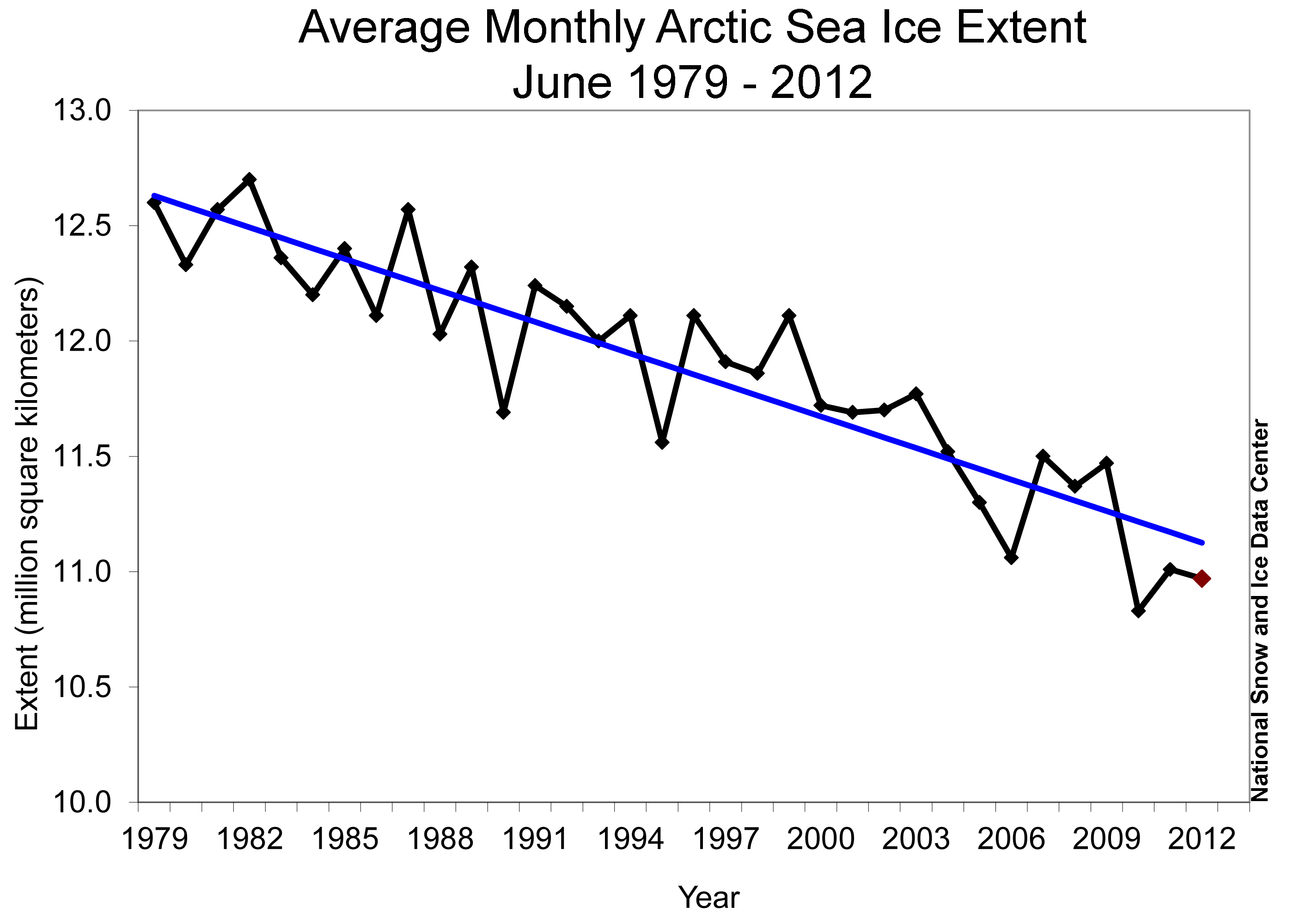
In terms of longer, climatological trends, Arctic sea ice extent in July has decreased linearly by 7.1% per decade. This rate is lowest in the spring months and highest in late summer/early fall months. Note that this rate also uses 1979-2000 as the climatological normal. There is no reason to expect this rate to change significantly (more or less negative) any time soon. Additional low ice seasons will continue. Some years will see less decline than other years (like this past year) – but the multi-decadal trend is clear: significantly negative. The specific value for any given month during any given year is, of course, influenced by local and temporary weather conditions. But it has become clearer every year that humans helped establish a new normal in the Arctic with respect to sea ice. This new normal will continue to have far-reaching implications on the weather in the mid-latitudes, where most people live.
Arctic Pictures and Graphs
The following graphic is a satellite representation of Arctic ice as of July 7, 2012:
Figure 1 – UIUC Polar Research Group‘s Northern Hemispheric ice concentration from 20120707.
Compare this with August 6th’s satellite representation, also centered on the North Pole:
The sea ice in the Canadian archipelago and along the northern coast of Russia determine whether the Northwest and Northeast passages open up or not. You can see by comparing the two graphs that the ice is nearly completely melted in the Canadian archipelago. The ice is also mostly melted along the entire northern coast of Russia – just a little remains in the Eastern Siberian sea. Last year, both passages opened again. I continue to think that the Northern Passage will likely open sometime this month. The Northeastern Passage might not open this year, but if it doesn’t, it won’t do so by a thin margin. You can also see in Figure 2 that the dominant wind direction has been toward Greenland. This allows ice to stack up against a landmass and not be exported as quickly out into the Atlantic Ocean where it is likelier to melt. The aforementioned Arctic Ocean storm has shifted wind direction somewhat across the basin, so I don’t expect all of the ice in Figure 2 to remain come September.
Overall, the health of the remaining ice pack is not healthy, as the following graph of Arctic ice volume from the end of July demonstrates:
Figure 3 – PIOMAS Arctic sea ice volume time series through July 2012.
As the graph shows, volume hit another record minimum in June 2012. Moreover, the volume is far, far outside the 2 standard deviation envelope (lighter gray contour surrounding the darker gray contour and blue median value). Figure 3 demonstrates how anomalous conditions are for sea ice in the Arctic. The volume has exceed the -4 standard deviation this year as well as the past two years. I understand that most readers don’t have an excellent handle on statistics, but conditions between -1 and -2 standard deviations are not very common; conditions outside the -2 standard deviation threshold (see the line below the shaded area on the graph above) are incredibly rare: the chances of 3 of them occurring in 3 subsequent years under normal conditions are extraordinarily low. Hence my assessment that “normal” conditions in the Arctic are shifting from what they were in the past few centuries: a new normal is developing. Note further that after conditions returned to near the -1 standard deviation envelope in late 2011/early 2012, as it did in early 2011, volume has once again fallen rapidly outside of the -2 standard deviation area. That means that natural conditions are not the likely cause; rather, another cause is much more likely to be responsible for this behavior.
I found a new graph that shows this and some additional information in a slightly different way:
Figure 4 – PIOMAS Arctic Sea Ice Volume from 1980 through July 2012.
This figure shows volume as a function of date. 2012 is the red curve, which is plotted against the average volume of 2010 through July 2012 (yellow), the average volume of the 2000s (green), the average volume of the 1990s (blue), and the average value of the 1980s (violet). Individuals years from 1979-2011 are indicated by the light gray curves. It is once again clear how anomalous recent conditions are compared to conditions from the latter part of the 20th century. It further shows how rapidly conditions have changed: the volume differences implied by this graph are astounding. The minimum volume typically occurs in early September, which we are approaching again in 2012.
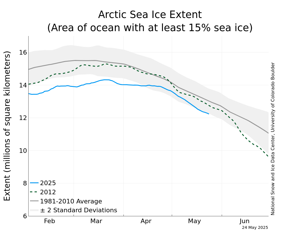
Switching back from volume to area, take a look at July’s areal extent time series data:
This is the time series graph that the NSIDC occasionally includes in their monthly reports. I present only this graph and not the graph updated daily throughout the month because of the historical context this graph provides. The ice that piled up in the winter wasn’t thick enough to prevent rapid melt to occur (see early June 2012). The effect of the thickening over the winter on September’s minimum extent will indicate how helpful the early season winds were in building sea ice that doesn’t melt every year back up. Right now, the situation doesn’t look good for September extent. During June, as I wrote above, melting occurred at record rate, resulting in a return to record low extent conditions by the middle of June. 2012′s extent has been below 2007′s for over two months and has been challenging all-time daily record minimums for almost two months. You can also see in this time series graph that conditions since 2007 have clearly differed from the normal conditions established from 1979-2000 (light gray contours surrounding the dark gray mean value).
Figure 6 – NSIDC northern hemisphere sea ice area (not extent) from the past two years only (blue) and the 1979-2008 mean (gray). The red curve shows the anomaly from the mean.
Note in Figure 6 how low the sea ice area is in the beginning of August 2012: -2.157 million sq. km.! Note two additional things. 1) The 2012 area value already is less than the climatological mean value by ~1.5 million sq. km. 2) The 2012 area value is only ~0.5 million sq. km. higher than the minimum recorded in 2011. The area value has slid just slightly under 3 million sq. km. only twice before: 2007 and 2011. Unless weather conditions change radically in the next couple of weeks, 2012 is also very likely to witness another sea ice area value under 3 million sq. km. The link above also shows that sea ice area was lower than 4 million sq. km. only during the past 5 years. Back in the 1980s, the area didn’t fall beneath 5 million sq. km. except for two years (1984, 1989). This is simply another way of noting that the Arctic environment has changed substantially in the past generation. One more note about the anomaly value (-2.157 here): 2007’s lowest anomaly currently ranks as the modern-day record: -3.6 million sq. km. 2012’s anomaly value is obviously far away from that, but has spent the most time below -2 million sq. km. than any year except 2007.
Antarctic Pictures and Graphs
Here is a satellite representation of Antarctic sea ice conditions from July 7th:
Ice gain is less easily visible around the continent than it was a few months ago. As a reminder, the difference between long-term Arctic ice loss and lack of Antarctic ice loss is largely and somewhat confusingly due to the ozone depletion that took place over the southern continent in the 20th century. This depletion has caused a colder southern polar stratosphere than it otherwise would be, reinforcing the polar vortex over the Antarctic Circle. That vortex has helped keep cold, stormy weather in place over Antarctica that might not otherwise would have occurred to the same extent and intensity. As the “ozone hole” continues to recover during this century, the effects of global warming will become more clear in this region, especially if ocean warming continues to melt sea-based Antarctic ice from below. For now, we should perhaps consider the lack of global warming signal due to lack of ozone as relatively fortunate.
Finally, here is the Antarctic sea ice extent time series from August 6th:
Antarctic sea ice extent had remained at or above average to some extent through the late austral fall and through the austral winter, which is good news. The difference in conditions from the first part of 2011 to the similar time period in 2012 is obvious: NSIDC measured last July’s extent near the bottom of the standard deviation envelope while this year’s extent is much healthier.
Errata
Here are my State of the Poles posts from July and June.
Ernesto underwent some intensification today, reaching hurricane strength as of the most recent advisory update from the National Hurricane Center. Within the next 12 hours, Hurricane Ernesto will make initial landfall along the Mexican coast, north of Belize. He is predicted to spend just under 24 hours moving over Mexico (weakening to a Tropical Storm) before re-emerging over the warm southern Gulf of Mexico waters. Just over one day later, Ernesto will likely make second landfall along the Mexican coast (likely re-strengthening to a hurricane).
Hurricane Ernesto’s center is currently located near 18.8N 86.2W; has a central minimum pressure of 983mb; has maximum sustained winds of 80mph; and is moving WHW @ 15mph. Hurricane Ernesto has a very good satellite appearance with concentric outflow and cold cloud-top temperatures:
Hurricane Ernest is predicted to continue moving generally westward, then curving slightly south of west over the next five days:
I’ve written a couple of posts on climate change basics (Gases, Forcing & Surface Temperature and Energy & Projections) that described how energy enters and moves through the climate system and some physical ramifications of emitting greenhouse gases. This post will build on those in an important way by examining what is very likely to happen to the base climate system in response to increasing carbon emissions. The operative word that is used throughout is: permanency. The climate system has so far been slightly altered by our species’ emissions. Most of the effects of that alteration won’t go away for hundreds of years. As humans emit additional emissions, the effects grow.
For all intents and purposes, as far as our species is concerned, the climate system’s alteration will not go away for a long, long time – on the order of thousands of years. That’s permanency as far as we’re concerned. Or, as the paper I cite puts it: it’s irreversible. Conditions will very likely not return to those we’ve experienced in our lifetimes and in the past few thousand years for many thousands of years into the future. That’s the cold, hard scientific truth of the situation. Now, people can decide for themselves whether such irreversibility or permanency is a “good” or “bad” thing – I won’t make normative judgments for anyone else but myself. I don’t consider such a change a “good” thing. The effects I will describe here are significant, but they are only those that are easily projected. Many other effects that haven’t been considered or experienced by our species will almost certainly fall out as a result of projections discussed here. Our civil institutions are not well equipped to handle even the first-order effects, let alone the compounding influence of effects upon effects.
On a personal note, I will not describe things as ‘catastrophic’ anymore. I have hinted at this in some posts I’ve written in the past few months without much explanation. The primary reason for this is using such language simply turns people off from considering the material. I think we need more people engaged on this topic, not less, and will consider scientific results of language and framing as much as I consider climate science results (a post dealing with this specifically is in the works). That said, I will continue to not spend many resources to engage the ideologically driven skeptic community. They simply have a different worldview than I do and neither party will convince the other that their side is “correct”. One goal of this blog is to inform those who are interested and to have civil, productive discussions of peer-reviewed climate science and the political/policy implications of that science.
So, before I delve into some details, words like `permanency` and `irreversible` will be used more frequently on this blog in the future. I will not use words like catastrophic. On that note…
Susan Solomon and her coauthors published a paper in 2008 entitled, “Irreversible climate change due to carbon dioxide emissions.” The primary finding: climate change resulting from anthropogenic carbon dioxide emissions is largely irreversible for 1,000s of years after the emissions stop. As a result, atmospheric temperatures are likely to remain higher than present-day values, rainfall reductions during dry seasons are likely to occur across the planet, and sea level rise is likely to continue to occur for thousands of years even though the models they used did not include every physical process involved in the hydrologic cycle in addition to the noted lack of all first-order forcings. The study gives us an idea of the type of temperature trends we are likely to experience for the next few thousand years as well as a conservative estimate of how high average global sea level rise will be.
In similar fashion as other modeling work, Solomon et al. allow CO2 concentrations to rise, then halt suddenly at some level in the future (reflecting a dramatic shift in human behavior such as radical technological innovation, etc. I characterize this treatment of behavior as “magical” because there is never robust reasoning to adequately describe such behavior shifts). Concentrations in the study rose at 2%/year to peak CO2 values of 450, 550, 650, 750, 850, and 1200 ppmv, followed by zero emissions after hitting each peak. For reference, current annual CO2 concentrations average just over 390pppmv. What occurs after the peaks is the interesting part of this paper, as the following graph shows:
The x-axis shows time in years out to the year 3000. Pre-industrial CO2 concentrations are indicated by the dashed line near the bottom of the graph. Without any effort at emissions’ mitigation, any one of these peaks is well within the realm of possibility. What happens after each peak? An extended period of time during which CO2 concentrations remain much higher than pre-industrial levels. Concentrations remain at levels between ~300 to ~800ppmv for the next thousand years, decreasing at decreasing rates during and after they reach their respective peaks. What effect might this have on temperature? The next graph in the paper demonstrates the simulated effects:
Each curve in this graph corresponds to the emissions lines in the previous graphs. Temperatures remain at least 1°C warmer (and up to 4°C warmer) than those of the year 1800 for the next thousand years. Temperatures do not decline at nearly the rate that CO2 concentrations do in the latter part of the millenium. While CO2 concentrations remain higher throughout the period, “permanency” is evident by temperature trends through the year 3000. What does that mean for the real world? Whatever temperature shift takes place through the end of rising emissions stays in place for all intents and purposes for our species permanently.
Rising temperatures have many other effects on different earth systems, including sea levels. Here are the sea level change projections from the Solomon et al. study:
Again, each line in this plot corresponds to an emissions scenario and a temperature trace in the two previous plots. Note the y-axis on this plot: it only shows sea level rise due to thermal expansion. Any additional water entering the world’s oceans resulting from melting glaciers or land-based ice sheets are not included in this projection. Therefore, the reader can interpret this plot as a minimum of sea level rise through 3000. The greatest rise obviously corresponds to the highest emissions scenario and the highest temperature rise. 0.4m rise in the minimum projected by this study and 1.9m is the maximum. Similarly to the previous plots, sea level doesn’t decrease once emissions and temperatures stabilize. Instead, they continue to slowly increase throughout the next millenium and remain high in essence in a permanent sense.
What’s obviously inaccurate with this study is the instantaneous cessation of CO2 emissions. Many studies treat future emissions in similar fashion. How emissions decrease in the future is of course a large unknown and therefore impossible to model with high accuracy. Solomon et al. do acknowledge that their treatment of emissions is not meant to be realistic, but to “represent a test case whose purpose is to probe physical climate system changes”. The primary lesson from this paper is relevant no matter the specific future emissions pathway: the longer emissions continue at any level close to 20th century levels, the longer it will take before concentrations stop rising and begin their slow descent in a planet with full carbon sinks, and temperatures and sea levels stabilize. The point at which all of these conditions peak is, in the end, almost entirely up to us.
The policy implications of this and other studies are obvious and not-so-obvious. Among the former: the willingness of coastal residents to incur higher infrastructure and other costs in future years versus their desire to implement policies designed to mitigate their situation; the willingness of non-coastal residents to keep funding federal insurance programs that allow others to live in high-risk zones; the way in which municipalities write zoning laws: for developers or for citizens; policy development that will help populations adapt to climate change effects in their region and/or that address mitigation on a larger scale; the priority assigned to programs that may or may not generate technological innovations that would lead to adaptive or mitigative strategies at some undefined point in the future (via government or business); how to address the need that policymakers have for information that will facilitate a balanced approach between short-term gain and long-term risk management. Other implications exist, as I’m sure most readers can attest. One result of this study is clear: we have locked in a certain amount of costs just as we’ve locked in a certain amount of warming and subsequent changes in multiple earth systems.
On the heels of the warmest July in Denver’s history, the first five days of August were also warmer than normal. Due to a cool front that made its way through the metro area Friday night, Saturday’s high temperature was only 83°F. Sunday was just as warm as Friday, however, with highs of 97°F and 98°F, respectively.
Through the first five days of the month, the average high has been 93.0°F. The average temperature over those five days was 77.1°F – a clear reflection of how relatively cool Saturday’s temperatures were. The departure from normal tracked above 4°F, but is only 2.7°F now. You can bet that departure reading will edge back up toward 4°F given the lack of weather systems on the horizon.
I still think Denver’s 100°F+ days are likely over for 2012. Despite my knowledge of future climate projections for the area, I sincerely hope 100°F+ days remain rare in my personal future. As many other cities across the US can attest, 100°F+ days are simply miserable, in addition to being dangerous to people’s’ health.
The Denver area continues to experience Severe to Extreme drought conditions (see figure below). I don’t think the last week’s rains will make a serious dent in those conditions.
Figure 1. Drought conditions across Colorado as of July 31, 2012. The orange contour indicates Severe drought conditions; the red contour indicates Extreme drought conditions; the brick-red contour indicates Exceptional drought conditions.
In the past couple of weeks, conditions have shifted spatially but haven’t worsened substantially. Some areas have actually seen slight relief from Extreme to Severe conditions. This is a shift from three months ago when, as the table in the figure shows, 0% of the state experienced Extreme conditions while 65-73% of the state experienced similar conditions in the past two weeks. Weather conditions over the next few weeks will determine the level of drought the state experiences.
Consecutive 90°F-day streaks
Saturday’s high of only 83°F (which felt fantastic!) also stopped the streak of consecutive 90°F+ days from early July through early August at 24. Once the NCDC confirms the temperatures, this streak will match the longest streak in Denver’s history, first set from July 13th through August 5th, 2008. Denver’s earlier streak of 15 consecutive 90°F+ days should tie for 5th on the all-time list.
Total 90°F+ Days
The record for total 90°F+ days in one calendar year is also in serious trouble. Through the 5th of August (yesterday), Denver had already recorded 50 such days in 2012 (2 in May, 17 in June, 27 in July, and 4 in August). That is enough days to tie for 9th on the all-time list. It seems incredible to someone who has lived in the area for a long time, but the all-time record of 61 90°F+ days seems easy to reach at this point in 2012. Denver has already surpassed 90°F today, and the NWS predicts similar highs for the next four days. That will mark 55 90°F+ days, good for a tie for the 4th most 90°F+ days and only 6 days from the all-time mark. The GFS model provides a glimpse for days beyond Friday and the pattern might change over the upcoming weekend: 90°F is the forecasted high for both days. Given recent history, I can easily envision highs of 91°F or 92°F, but I look forward to days that can no longer climb above 90°F.
T.S. Ernesto’s center is located near 15.8N 80.5W; has a central pressure of 994mb (and falling); has maximum sustained winds of 65mph; and is now moving WNW at only 9mph.
T.S. Ernesto is predicted to steadily strengthen over the next 48 hours and top out with 90mph sustained winds. He should reach hurricane strength sometime in the next 24 hours. While over Belize and southeastern Mexico, Ernesto will weaken. There is a chance the storm will re-emerge over the southern Gulf of Mexico and regain some of its strength before making a second landfall over the eastern coast of Mexico near the southwestern Gulf of Mexico. Thereafter, the storm will dissipate over the Mexican landmass.
Figure 1. NHC’s map of Ernesto’s current position and likely future track and intensity forecast as of 2P EDT on 20120806. Circles with H’s indicate hurricane strength; with S’s indicate tropical storm strength; with D’s indicate tropical depression strength.
Unfortunately, there will not be any potential for short-term drought relief by Ernesto over the US. Mexico will benefit from its likely prodigious rainfall, however.
The storm complex that was Florence will gradually turn toward the northwest over the next five days, remaining well out to sea. Recall that this was a Cape Verde storm and this track and behavior is common for these type of storms: they simply form too far east to have any impact on any Western Hemispheric landmasses.
Other Potential Storms
Another tropical wave has transited Africa, but this wave is much weaker than Ernesto or Florence was. The next tropical wave is just west of central Africa and should enter the Atlantic Ocean in a few days’ time. No other tropical development is likely in the next week.


