First, a little historical perspective. Global mean sea levels rose in the 20th and 21st centuries: about 0.2m. Prior to research conducted in the past five years, projections of additional 21st century sea-level rise ranged from another 0.2m to 2.0m. These projections did not, in general, consider feedbacks; the parent simulations did not consider cryosphere processes (i.e., melting glaciers and the land-based Greenland and Antarctic ice sheets). More recent research included more feedbacks and cryosphere processes, but their treatment remains immature. Additionally, recent research started to examine projections based on realistic emissions scenarios, after researchers began to accept the fact that policymakers are unlikely to enact meaningful climate policy any time soon. As such, sea-level projection ranges increased. Which is where this latest paper comes in.
Levermann et al. reported a 2.3 m/°C sea-level rise projection in the next two thousand years. Benjamin Strauss’s PNAS paper put this into context:
[W]e have already committed to a long-term future sea level >1.3 or 1.9m higher than today and are adding about 0.32 m/decade to the total:10 times the rate of observed contemporary sea-level rise
Thus, if global temperatures rise only 1°C and stabilize there (an extremely unlikely scenario), sea-levels two thousand years from now could be 2.3 m higher. This might not sound like much, but an additional 7.5 feet of sea level rise would inundate 1.5 million U.S. peoples’ homes at high tide. With 2°C, sea levels could rise 4.6m. On our current emissions pathway, global mean temperatures would rise 4°C, which would result in an additional 9.2 m of sea level rise. That’s 30 feet higher than today! Levermann notes that these higher sea level projections are supported by sea level heights that occurred in the distant past (paleoclimate), even with their associated uncertainties.
And now a couple of important points. Some of the processes Levermann utilized involved linear change. In complex systems like the Earth’s climate, very few changes are linear. Many more are exponential. When I discuss linear and exponential change with my students, I include a number of different examples because our species doesn’t easily understand exponential change. We typically severely underestimate the final value of something that changes exponentially. If changes within the climate system occur exponentially, the Levermann projections probably won’t be valid. But their estimate will likely be an underestimate.
A USA Today article on the Levermann paper has this quote:
Looking at such a distant tomorrow “could scare people about something that might not happen for centuries,” says Jayantha Obeysekera of the South Florida Water Management District, a regional government agency. He says such long-term projections may not be helpful to U.S. planners who tend to focus on the next few decades.
Should people be scared that their communities will be underwater in 2000 years? I don’t think they will be, number one. Few people pay attention to trends that will affect them in 2 or 20 years. 200 or 2000 are well beyond anybody’s individual concern. But I think society as a whole should examine this updated projection. Do we want to condemn one-third of Florida to the bottom of the Atlantic Ocean? Do we want to condemn thousands of towns and cities to that fate, even if the time horizon may be well beyond our lifetime?
Moving beyond the inevitable question regarding fear, what do these results mean? We need to include results like these in planning processes. If nothing else, planners and policymakers have more realistic estimates of likely future sea level in hand. Those estimates will continue to change (hopefully for the better) with additional research. But decision-making shouldn’t stop with the expectation that some future projection might be perfect because it won’t be. The decisions we make today will have profound effects on the eventual level of the sea in the distant future. There will also be countless effects on the climate, societies, and ecosystems until we reach that level. That is what today’s decision-making needs to address.
Climate Central has a useful map to investigate how potential thresholds implicate sea level rise with respect to US states at different points in the future.
The fourth named storm of the 2013 Atlantic hurricane season formed earlier this week off the west coast of Africa. T.S. Dorian is moving west under the influence of a strong mid-level ridge. He encountered cool sea-surface temperatures a couple of days ago. While over warming waters since then, high vertical wind shear and dry, stable air to his north encumbered him since then, which kept his strength at Tropical Storm status. Dorian is a compact tropical system and currently has no banding features on satellite imagery.
The National Hurricane Center’s official track forecast keeps Dorian south of 20N through the weekend as he approaches the Lesser Antilles from the northeast. By Monday morning, the NHC’s current forecast has Dorian north of Puerto Rico as a Tropical Storm. The forecast then shows Dorian north of the Dominican Republic Tuesday morning and just off-shore eastern Cuba Wednesday morning. By Wednesday, the track uncertainty cone extends from Jamaica (south of Cuba) to the Bahamas (north of Cuba and east of southern Florida). The official intensity forecast keeps Dorian at Tropical Storm strength through Wednesday.
Any impacts to the United States, if there are any, will not occur until the second half of next week.
Australia voted last week to scrap their carbon tax and replace it with a much less economically efficient cap-and-trade scheme. The pro-business Reuters article acknowledges the only “positive” that results from this decision: businesses will save money. Well, hallelujah. I’m sure today’s children will be immensely grateful when they’re adults with all the resultant climate change effects that Australian businesses were able to avoid paying for their actions and saved a few billion dollars in the 2010s. That’s one way to look at this news. Let’s flesh the landscape out before throwing Australia under the bus too quickly.
To be fair, Australia simply moved up the date when they joined … the European carbon “market”. You remember, that’s the market that severely over-supplied carbon credits at its outset and refused earlier this year to remove some of those excess credits for a mere two years. In essence, the European carbon market doesn’t work. How can you tell? Carbon costs €4.2/tCO2 today. When the European market started, the cost was €31/tCO2. At one-tenth the original price, the market signal is clear: there are far too many allowances in the European market. Have greenhouse gas emissions (note: CO2 isn’t the only GHG!) fallen in the EU since the market’s inception? Yes, but this is a result of the continued economic malaise the Europeans inflict on themselves, as described by the European Environment Agency’s most recent report.
The temporary benefit to the earlier Australian move to the EU’s ETS is this: the flow of carbon credits is one way: from Europe to Australia. Australia can’t export credits until July 2018. So in the short-term, Australia could help relieve the over-supply of EU carbon credits. This might help in raising the carbon price back to more realistic levels, but this won’t happen until 2016 at the earliest because of lower emissions and demand for permits in Australia.
There are two big negative effects of moving from a fixed tax to a floating market. The first is that carbon will become much cheaper in Australia: from A$25.40 per tonne to A$6 per tonne. Is carbon really only worth A$6? In an over-supplied market, perhaps it is. The fact that not all industries are involved in the carbon market means that we manipulate the true carbon price. Of course, as much as folks like to talk about “free markets”, most markets are heavily manipulated by vested interests. The second negative effect remains local: the move removes A$3.8 billion from the Australian federal budget over four years. Australia’s Prime Minister Kevin Rudd proposed to make up this budget shortfall by “removing a tax concession on the personal use of salary-sacrificed or employer-provided cars.” Good luck with that, Mr. Rudd. Everybody is loath to give up a financial benefit once they receive it. Look – more market manipulation!
Australian coal companies were more than happy to propagate misinformation to Australian energy consumers: electricity price increases were due exclusively to the carbon tax! This highlights a common problem with any carbon-pricing scheme: special interests can more easily spread misinformation and disinformation (and are often happy to do so!) than market proponents can spread true information. The reason is often quite simple: the truth is complex and consumers don’t want to invest the time to understand why they pay the prices they pay. How many consumers demanded energy utilities stop raising prices before carbon market inception? Then who was responsible for price increases? “Market forces” is the lame excuse dished out to the masses. How about the relentless, unquenchable hunger for ever-rising profits? Somehow, that’s alright, but accurately pricing a commodity is heresy.
An additional piece of context: Australia suffered from record heat waves, droughts, and floods in the past ten years. The Australian public’s acceptance of climate change related to these disasters is widespread, as is their desire to “take action”. Well, the government took action and that same public cried uncle with slightly higher utility bills. This proves the common refrain: people support climate policies … so long as they are absolutely free. That smacks into reality awfully quick. It also demonstrates that there is no such thing as a “Climate Pearl Harbor” that leads to unequivocal support for a given climate policy. The slow-acting nature of climate works strongly against widespread, effective climate policy.
A substantial portion of the U.S. population experienced a heat wave during the past week. Due to the number of people affected, the media spent some time on the topic. As opposed to places like Las Vegas or Phoenix, where the “heat is supposed to happen”, folks normally accustomed to rather pleasant summer conditions experienced real heat again. Heat waves of various intensity happen every year. This heat wave is rather intense – it is breaking some heat records. Some interesting factoids:
Temperatures at Newark Liberty Airport in New Jersey were recorded at 98 degrees at 1 p.m. local time on Friday, as the mercury hit 93 in Central Park. John F. Kennedy Airport in Queens, New York, recorded temperatures of 100 degrees on Thursday, beating out the previous record set for that date a year ago, and on Friday the heat index there reached 108.
Electricity usage soared to an all-time high in New York City as the work week closed out, provider Con Edison announced, as service hit a peak of 13,214 megawatts around 2 p.m. local time. The previous record was 13,189 megawatts on July 22, 2011, according to the company.
So, some serious heat and serious energy consumption. The latter proves interesting to look at in more detail: if warming trends continue, power plants will be unable to operate like we expect them to due to water and infrastructure cooling requirements. That spells trouble for people: the worst heat waves of the future might be accompanied by temporary brownouts and blackouts. How manageable will heat waves be with no A/C?
What about the warming trend? If we stay on our current greenhouse gas emissions pathway (the highest considered by climate models), look at the potential number of weeks with 100°F+ temperatures in 2090-2099:
Figure 1. Projection of A1FI emissions pathway-derived number of weeks (2090-2099) per with daily maximum temperatures exceeding 100°F.
With this heat wave fresh in mind, imagine what it will be like later this century when there is more than one excessive heat wave per year in the Midwest and along the east coast. Instead of five days of misery, what will 25 days be like? How about 50 days of 100°F heat in Virginia, North Carolina, Kentucky, Illinois, Iowa, and Nebraska? When 100°F daytime heat dominates one, two, or even three months every year and high nighttime temperatures accompany it, this week’s heat wave will seem refreshing by contrast.
That’s how we feel in Denver, CO this year. Instead of 73 total 90°F+ days – 13 of those days at 100°F+ – in 2012 (with June 2012 7.6°F warmer than normal), summer 2013 has been closer to average. Yes, it’s been warm and only one 100°F day occurred so far this year, but it feels almost pleasant in comparison to last summer when the heat was relentless for months on end.
Three days of excessive heat is difficult to experience. Three months is currently unimaginable. How much worse future heat waves get is mostly within our control. The sooner we significantly cut greenhouse gas emissions, the better things will end up for all of us. But as the above graph demonstrates, the future could be quite hot if we continue along our current emissions pathway too much longer.
The Denver Post Editorial Board took a stance on car mileage based on a recent Consumer Reports (CR) article. Let me state at the outset that I regularly use Consumer Reports rankings as part of my purchase decision-making process. That said, no testing is ever 100% complete and is much less regularly communicated well to non-experts. At issue: CR performed independent tests on cars and calculated different miles per gallon values than those the EPA provided. Should the EPA update their testing? Perhaps, but the Editorial Board and CR didn’t provide an overwhelming case to do so. Let’s look at what each entity said.
First, the Post:
Consumers could very well feel deceived by the numbers, but there are other issues at work.
Hybrids with just a single occupant can zip past traffic using high-occupancy-vehicle lanes in some parts of the country — including Colorado — because of their superior efficiency. The idea is to support, through public policy, efficient vehicles that generate less harmful emissions. But if they’re really not substantially more efficient, it’s neither environmentally beneficial nor fair to drivers of traditional vehicles that may, in reality, get similar gas mileage.
There are key parts to this section that I want to highlight. What does “substantially more efficient” mean? What value efficiency is enough to warrant public policy? In the Denver area, suburban drivers love their SUVs and trucks. So to start, I’ll compare an SUV, a truck, a sports car, and a 2010 Prius. And I’ll start with the location the Board identified as a policy recipient: the highway. The EPA’s ratings for these four vehicles are: 15, 18, 26, and 48mpg (highway). Should Prius drivers receive plicy support for driving a vehicle that averages 2-3X as many mpg as the majority of other vehicles?
Let’s change the argument a little to better match the spirit of the article and consider the “combined” fuel efficiency. This designation accounts for street driving and highway driving. The same four vehicles have the following combined ratings: 13, 14, 21, and 50mpg. The complaint that CR and the Board has is the hybrid value is too high (based on their own testing protocols, which aren’t detailed very well). So let’s change the hybrid’s EPA combined value with CR’s “overall” value: 44mpg. Should we direct public policy toward cars that get 2-3X as many mpg as the majority of other vehicles? Note that the comparison, and thus my argument, didn’t change.
The argument that CR made is that their hybrid vehicle test values differed from EPA values by more than 3mpg on average. Yes, 6mpg is a difference. Are consumers being tricked? I don’t think so. And this is really where I split with CR. Here is their take:
Overall, fuel-efficiency shortfalls have narrowed considerably over the years. When Consumer Reports conducted a similar study in 2005 that compared our gas-mileage results with the EPA estimates, we found that most cars got significantly fewer mpg than their window stickers promised. Conventional gas-powered vehicles missed their EPA estimates by an average of 9 percent, and hybrids by 18 percent.
So it isn’t as if CR is bashing hybrids; far from it. All of the EPA sticker values differed from CR’s. That isn’t surprising since CR tested vehicles differently. One vital question: which test best mimics real-world driving? Most people drive very aggressively (hard acceleration and braking), which has a big impact on gas mileage. Are the CR values too high? What if we consider additional factors: heat and cold, wind and rain. Those happen in the real world. But not in the CR tests. Isn’t it interesting that a consumer advocacy group is challenging the EPA’s tests for being unrealistic when they themselves didn’t test vehicles in real-world conditions? How far off are CR’s values? We don’t know. Should we reengineer public policy in the face of CR’s unrealistic tests? For what purpose? Should the EPA and CR develop a more rigorous testing protocol – perhaps one that both entities can perform and therefore directly compare against one another?
I have another problem with the CR quote. Note the bolded words. EPA doesn’t promise drivers that they’ll attain the sticker mileage. In fact, the EPA goes out of its way to emphasize and explain their values are merely estimates. That’s not a promise, not even close. It’s annoying that people read too much into things. In fact, CR could do what I did: check the EPA website for common misconceptions. The ninth most common:
9. The EPA fuel economy estimates are a government guarantee on what fuel economy each vehicle will deliver.
The primary purpose of EPA fuel economy estimates is to provide consumers with a uniform, unbiased way of comparing the relative efficiency of vehicles. Even though the EPA’s test procedures are designed to reflect real-world driving conditions, no single test can accurately model all driving styles and environments. Differing fuel blends will also affect fuel economy. The use of gasoline with 10% ethanol can decrease fuel economy by about 3% due to its lower energy density.
Like I said, the EPA goes out of its way to explain what its published values are. CR and the Board should have done 60 seconds of checking before they called out the EPA for deceiving consumers with “promises”.
A more appropriate target are auto manufacturers, who know what the tests are and try their best to optimize the results. The same entity that has a financial interest in optimizing estimated mileage should not test vehicles’ mileage. Like I wrote above, this is where CR and EPA should work together to independently test vehicles.
But as far as the basic argument goes, hybrids do get better overall mileage than other vehicles. They get the best mileage if drivers drive them where manufacturers intended them to drive: in stop-and-go city traffic. But they still drastically outperform their competition in highway driving, enough so that I think current public policies provide nearly the correct incentive for drivers to think of another dimension when choosing which vehicle they will purchase.
According to the Drought Monitor, drought conditions improved recently across some of the US. As of Jul. 9, 2013, 47.3% of the contiguous US is experiencing moderate or worse drought (D1-D4), as the early 2010s drought continues month after month. That is the lowest percentage in a number of months. The percentage area experiencing extreme to exceptional drought increased from 14.6% to 14.8%, but this is ~4% lower than it was six months ago. The eastern third of the US was wetter than normal during June, which helped keep drought at bay. The east coast in particular was much wetter than normal. Instead of Exceptional drought in Georgia and Extreme drought in Florida two years ago, there is flash flooding and rare dam water releases in the southeast. Eight eastern states experienced their top-three wettest Junes on record. The West is quite a different story. Long-term drought continues to exert its hold over the region, as it remains warmer and drier than normal month after month.
If we focus in on the West, we can see recent shifts in drought categories:
Figure 2 – US Drought Monitor map of drought conditions in Western US as of July 9th.
Early year snowmelt relief was short-lived, as drought conditions expanded as worsened in the past three months. More than three-fourths of the West is in Moderate drought. More than half of the West is now is Severe drought. And one-fifth of the West is in Extreme drought.
Temporary drought relief might occur in New Mexico and southern Colorado due to the recent heavy rains brought by a retrograding low pressure system that also brought cooler than normal temperatures to Oklahoma and Texas.
Here are the conditions for Colorado:
Figure 3 – US Drought Monitor map of drought conditions in Colorado as of July 9th.
There is some evidence of relief evident over the past six months here. Severe drought area dropped from 95-100% to 83%. Extreme drought area dropped significantly from 53% to 39%. Exceptional drought shifted in space from central Colorado to southeastern Colorado, which left the percentage area near 17%. The good news for southeastern Colorado is the recent delivery of substantial precipitation. It isn’t likely to alleviate the long-term drought, but will hopefully dent short-term drought.
US drought conditions are more influenced by Pacific and Atlantic sea surface temperature conditions than the global warming observed to date. Different natural oscillation phases preferentially condition environments for drought. Droughts in the West tend to occur during the cool phases of the Interdecadal Pacific Oscillation and the El Niño-Southern Oscillation, for instance. Beyond that, drought controls remain a significant unknown. Population growth in the West in the 21st century means scientists and policymakers need to better understand what conditions are likeliest to generate multidecadal droughts, as have occurred in the past.
As drought affects regions differentially, our policy responses vary. A growing number of water utilities recognize the need for a proactive mindset with respect to drought impacts. The last thing they want is their reliability to suffer. Americans are privileged in that clean, fresh water flows every time they turn on their tap. Crops continue to show up at their local stores despite terrible conditions in many areas of their own nation (albeit at a higher price, as found this year). Power utilities continue to provide hydroelectric-generated energy.
That last point will change in a warming and drying future. Regulations that limit the temperature of water discharged by power plants exist. Generally warmer climate conditions include warmer river and lake water today than what existed 30 years ago. Warmer water going into a plant either means warmer water out or a longer time spent in the plant, which reduces the amount of energy the plant can produce. Alternatively, we can continue to generate the same amount of power if we are willing to sacrifice ecosystems which depend on a very narrow range of water temperatures. As with other facets of climate change, technological innovation can help increase plant efficiency. I think innovation remains our best hope to minimize the number and magnitude of climate change impacts on human and ecological systems.
During June 2013, the Scripps Institution of Oceanography measured an average of 398.58 ppm CO2 concentration at their Mauna Loa, Hawai’i Observatory.
This value is important because 398.58 ppm the largest CO2 concentration value for any June in recorded history. This year’s June value is 2.81 ppm higher than June 2012′s! Month-to-month differences typically range between 1 and 2 ppm. This year-to-year jump is clearly well outside of that range. This is more in line with February’s year-over-year change of 3.37 ppm and May’s change of 3.02 ppm. Of course, the unending trend toward higher concentrations with time, no matter the month or specific year-over-year value, as seen in the graphs below, is more significant.
The yearly maximum monthly value normally occurs during May. This year was no different: the 399.89ppm concentration in May 2013 was the highest value reported this year and, prior to the last five months, in recorded history (neglecting proxy data). I expected May of this year to produce another all-time record value and it clearly did that. May 2013′s value will hold onto first place all-time until February 2014.
Figure 1 – Time series of CO2 concentrations measured at Scripp’s Mauna Loa Observatory in June from 1958 through 2013.
CO2Now.org added the `350s` and `400s` to the past few month’s graphics. I suppose they’re meant to imply concentrations shattered 350 ppm back in the 1980s and are pushing up against 400 ppm now in the 2010s. I’m not sure that they add much value to this graph, but perhaps they make an impact on most people’s perception of milestones within the trend.
How do concentration measurements change in calendar years? The following two graphs demonstrate this.
Figure 2 – Monthly CO2 concentration values (red) from 2009 through 2013 (NOAA). Monthly CO2 concentration values with seasonal cycle removed (black). Note the yearly minimum observation occurred eight months ago and the yearly maximum value occurred last month. CO2 concentrations will decrease through October 2013, as they do every year after May.
Figure 3 – 50 year time series of CO2 concentrations at Mauna Loa Observatory (NOAA). The red curve represents the seasonal cycle based on monthly average values. The black curve represents the data with the seasonal cycle removed to show the long-term trend. This graph shows the recent and ongoing increase in CO2 concentrations. Remember that as a greenhouse gas, CO2 increases the radiative forcing of the Earth, which increases the amount of energy in our climate system.
CO2 concentrations are increasing at an increasing rate – not a good trend with respect to minimizing future warming. Natural systems are not equipped to remove CO2 emissions quickly from the atmosphere. Indeed, natural systems will take tens of thousands of years to remove the CO2 we emitted in the course of a couple short centuries. Human systems do not yet exist that remove CO2 from any medium (air or water). They are not likely to exist for some time. So NOAA will extend the right side of the above graphs for years and decades to come.
This month, I want to spend some more time on this focus: CO2 concentration values. Given our species’ penchant for round numbers, it came as little surprise that the corporate media placed an uncommon amount of attention on a value that really has relatively low meaning: daily CO2 concentrations at Mauna Loa surpassed 400 ppm for a day during the month of May. In fact, both the media and many climate activists made a very big deal about this development (news articles and my twitter feed “blew up” with this news). I think that was largely a waste of time. Again, the daily value itself didn’t represent any large difference once reached. The climate system did not automatically kick into a different setting once concentrations passed 400 ppm for a day. Nothing substantially new occurred that didn’t when concentration were “only” 399 ppm (or 390 ppm or 380 ppm for that matter). Indeed, where are the articles this month with daily values in the 398-399 ppm range? They’re nonexistent. So what is important: psychologically significant thresholds or the unending acceleration of concentrations across years and decades?
As I state in this series every month, the trend makes much more of a difference than any daily, monthly, or even yearly average value. And that trend is accelerating upwards at a rate that many experts didn’t think was possible even 10 years ago. The effects from last year’s average CO2 concentrations won’t manifest in real-world terms until 30-50 years from now. I didn’t see anybody else in May pointing out that important detail. Similarly, I didn’t see any explanation that today’s mean temperatures are largely a result of CO2 concentrations from 30+ years ago. Perhaps most importantly, climate activists didn’t mention that CO2 concentrations are rising at a rising rate despite decades of their “activism”. That fact creates a rather uncomfortable situation because most activists are proponents of doing tomorrow what they did yesterday. If those actions haven’t had any effect up until now, why the advocacy for the status quo when those same activists try to claim that the status quo is untenable. If they really believed in their catastrophic climate change claims, shouldn’t they honestly evaluate the effects their actions have had? And if those actions produced far less meaningful progress than they state is absolutely required for the survival of our species and the planet (grandiose language, I know), why do their strategies and tactics remain largely unchanged?
I write these posts for people who are curious or interested in the state of a key climate variable. Almost two years ago now, I realized that doomsday language turns a significant portion of my potential audience off from the get-go. If we are to do something meaningful about climate change, we cannot afford the disengagement and hostility of one-third or more of our fellow global citizens towards climate activism. I don’t want to simply treat people as empty vessels into which I can pour knowledge. I want to engage them on ground that is similar between us precisely because I want to do something. Screaming about a 400 ppm mean CO2 concentration for one day and then walking away from the variable until we pass the next perceived meaningful threshold doesn’t strike me as engagement.
The rise in CO2 concentrations will slow down, stop, and reverse when we decide it will. It depends primarily on the rate at which we emit CO2 into the atmosphere. We can choose 400 ppm or 450 ppm or almost any other target (realistically, 350 ppm seems out of reach within the next couple hundred years). That choice is dependent on the type of policies we decide to implement. It is our current policy to burn fossil fuels because we think doing so is cheap, although current practices are massively inefficient and done without proper market signals. We will widely deploy clean sources of energy when they are cheap; we control that timing. We will remove CO2 from the atmosphere if we have cheap and effective technologies and mechanisms to do so, which we also control to some degree. These future trends depend on today’s innovation and investment in research, development, and deployment. Today’s carbon markets are not the correct mechanism, as they are aptly demonstrating. But the bottom line remains: We will limit future warming and climate effects when we choose to do so.
During the month of June 2013, Denver, CO’s (link updated monthly) temperatures were 3.7°F above normal (71.1°F vs. 67.4°F). The National Weather Service recorded the maximum temperature of 100°F on the 11th and they recorded the minimum temperature of 39°F on the 2nd. Here is the time series of Denver temperatures in June 2013:
Figure 1. Time series of temperature at Denver, CO during June 2013. Daily high temperatures are in red, daily low temperatures are in blue, daily average temperatures are in green, climatological normal (1981-2010) high temperatures are in light gray, and normal low temperatures are in dark gray. [Source: NWS]
In comparison to April 2013, June 2013 brought less extreme weather to the Denver area. After a moderate start to the month’s temperature, high pressure began to dominate the area by the 11th through the end of the month. This high pressure brought warmer than average temperatures, which offset the early month cool snap. This same pattern brought warmer than average temperatures to much of the southwestern United States, culminating in extremely dangerous heat at the end of the month from Idaho to Arizona.
Denver’s temperature was above normal for the past two months in a row. May 2013 ended a short streak of four months with below normal temperatures. Seven of the past twelve months were warmer than normal. October broke last year’s extreme summer heat including the warmest month in Denver history: July 2012 (a mean of 78.9°F which was 4.7°F warmer than normal!).
Precipitation
Precipitation was lighter than normal during June 2013: only 0.75″ precipitation fell at Denver during the month instead of the normal 1.98″. Precipitation is a highly variable quantity though. The west side of the Denver Metro area received rainfall on days that the official Denver recording site did not, which is the usual case for convective-type precipitation.
Precipitation a couple of months ago alleviated some of the worst drought conditions in northern Colorado. The link goes to a late April 2013 post; further relief occurred in May with regular rain events. With below average precipitation in June for most areas, drought conditions unfortunately worsened during the month. All of Colorado continues under at least some measure of drought in early July 2013. The worst drought conditions (D4: Exceptional) continue to impact southeast Colorado however and the area with D4 conditions slowly expanded during the past few months. Absent a significant shift in the upper-level jet stream’s position, the NWS expects dry conditions to persist over CO during the next one to three months, which will likely worsen drought conditions. I will write an updated drought post within the week.
Interannual Variability
I have written hundreds of posts on the effects of global warming and the evidence within the temperature signal of climate change effects. This series of posts takes a very different look at conditions. Instead of multi-decadal trends, this series looks at highly variable weather effects on a very local scale. The interannual variability I’ve shown above is a part of natural change. Climate change influences this natural change – on long time frames. The climate signal is not apparent in these figures because they are of too short of duration. The climate signal is instead apparent in the “normals” calculation, which NOAA updates every ten years. The most recent “normal” values cover 1981-2010. The temperature values of 1981-2000 are warmer than the 1971-2000 values, which are warmer than the 1961-1990 values. The interannual variability shown in the figures above will become a part of the 1991-2020 through 2011-2040 normals. If temperatures continue to track warmer than normal in most months, the next set of normals will clearly demonstrate a continued warming trend.
Global polar sea ice area in June 2013 remained at or slightly above climatological normal conditions (1979-2008). This follows early 2013 conditions’ improvement from September 2012′s significant negative deviation from normal conditions (from -2.5 million sq. km. to +500,000 sq. km.). Early austral fall conditions helped create an abundance of Antarctic sea ice while colder than normal boreal spring conditions helped slow the rate of ice melt in the Arctic.
The NSIDC made a very important change to its dataset in June. With more than 30 years’ worth of satellite-era data, they recalculated climatological normals to agree with World Meteorological Organization standards. The new climatological era runs from 1981-2010 (see Figure 5 below). What impacts did this have on their data? The means and standard deviations now encompass the time period of fastest Arctic melt. As a consequence, the 1981-2010 values are much lower than the 1979-2000 values. This is often one of the most challenging conditions to explain to the public. “Normal”, scientifically defined, is often different than “normal” as most people refer to it. U.S. temperature anomalies reported in the past couple of years refer to a similar 1981-2010 “normal period”. Those anomalies are smaller in value than if they were compared to the previous 1971-2000 “normal period”. Thus, temperature anomalies don’t seem to increase as much as they would if scientists referred to the same reference period.
Arctic Sea Ice
According to the NSIDC, sea ice melt during June measured 2.10 million sq. km. This melt rate was slower than normal for the month, but June′s extent remained below average – a condition the ice hasn’t hurdled since this time last year. Instead of measuring near 11.89 million sq. km., June 2013′s average extent was only 11.5 million sq. km., a 300,000 sq. km. difference.
Barents Sea (Atlantic side) ice remained below its climatological normal value during the month, which continues the trend that began this last winter. Kara Sea (Atlantic side) ice temporarily recovered from its wintertime low extent and reached normal conditions earlier this year, but fell back below normal during May through June. Arctic Basin sea ice (surrounding the North Pole) fell below normal during June due to earlier weather conditions that sheared ice apart. The Bering Sea (Pacific side), which saw ice extent growth due to anomalous northerly winds in 2011-2012, saw similar conditions in December 2012 through March 2013. Since then, Bering Sea ice extent returned to normal for this time of year: zero. The previous negative Arctic Oscillation phase gave way to normal conditions throughout June. However, a stronger than normal Arctic Low set up which kept Arctic weather conditions cooler and stormier than normal. These conditions prevented Arctic sea ice from melting as quickly in June as it did in 2012. In the past few days, these conditions eased and rapid Arctic melt is once again underway. I’ll have more to say about this in next month’s post.
For the first time in a number of years, Arctic sea ice extent in June didn’t reach a bottom-ten status. June Arctic sea ice extent was “only” the 11th lowest on record. In terms of climatological trends, Arctic sea ice extent in June decreased by 3.6% per decade. This rate is closest to zero in the late winter/early spring months and furthest from zero in late summer/early fall months. Note that this rate also uses 1981-2010 as the climatological normal. There is no reason to expect this rate to change significantly (much more or less negative) any time soon, but negative rates are likely to slowly become more negative for the foreseeable future. Additional low ice seasons will continue. Some years will see less decline than other years (e.g., 2011) – but the multi-decadal trend is clear: negative. The specific value for any given month during any given year is, of course, influenced by local and temporary weather conditions. But it has become clearer every year that humans have established a new climatological normal in the Arctic with respect to sea ice. This new normal will continue to have far-reaching implications on the weather in the mid-latitudes, where most people live.
Arctic Pictures and Graphs
The following graphic is a satellite representation of Arctic ice as of June 13, 2013:
Continued melt around the Arctic ice periphery is evident in the newest figure. Hudson Bay ice is nearly gone. Rapid melt is also evident in the Kara, Barents, and Bering Seas. Compared to last year at the same time, more ice is present in the Baffin/Newfoundland, Beaufort, and Kara Seas. This is due to interannual weather and sea variability. The climate trend remains clear: widespread and rapid sea ice melt is the new normal for the Arctic.
So far, the early season thinning of sea ice near the North Pole hasn’t caused a mid-season mid-ocean collapse of sea ice, as many people feared. This is not to say that rapid ice melt in the central Arctic Ocean will not happen this year. We simply have to wait and see what happens before we issue obituaries.
The following graph of Arctic ice volume from the end of June demonstrates the relative decline in ice health with time:
Figure 3 – PIOMAS Arctic sea ice volume time series through June 2013.
As the graph shows, volume (length*width*height) hit another record minimum in June 2013. Moreover, that volume remained far from normal for the past three years in a clear break from pre-2010 conditions. Conditions between -1 and -2 standard deviations are somewhat rare and conditions outside the -2 standard deviation threshold (see the line below the shaded area on the graph above) are incredibly rare: the chances of 3 of them occurring in 3 subsequent years under normal conditions are extraordinarily low (you have a better chance of winning the Powerball than this). Hence my assessment that “normal” conditions in the Arctic shifted from what they were in the past few centuries; humans are creating a new normal for the Arctic. Note further that the ice volume anomaly returned to near the -1 standard deviation envelope in early 2011, early 2012, and now early 2013. In each of the previous two years, volume fell rapidly outside of the -2 standard deviation area with the return of summer. That provides further evidence that natural conditions are not the likely cause; rather, the more likely cause is human influence.
Arctic Sea Ice Extent
Take a look at May’s areal extent time series data:
Figure 4 – NSIDC Arctic sea ice extent time series through early July 2013 compared with five recent years’ data, climatological norm (dark gray line) and standard deviation envelope (light gray).
As you can see, this year’s extent (light blue curve) remained at historically low levels throughout the spring, well below average values (thick gray curve), just as it did in the previous five springs. Sea ice extent did something different this spring and early summer: the late season surge of ice formation seen in the 2009, 2010, and 2012 curves was not as strong this year; the early summer surge of ice melt seen in the 2010, 2011, and 2012 curves was also not as strong this year, at least not until the last week or so. This graph also demonstrates that late-season ice formation surges have little effect on ice extent minima recorded in September each year. The primary reason for this is the lack of ice depth due to previous year ice melt. I will pay close attention to this time series throughout June to see if this year’s curve follows 2012′s. Note the sharp decrease in sea ice extent in mid-June 2012. That helped pave the way for last year’s record low September extent, even though weather conditions were not as a factor as they were during the 2007 record low season.
Figure 5 – Graph comparing two climatological normal periods: 1979-2000 (light blue solid line with dark gray shaded envelope) and 1981-2010 (purple solid line with light gray shaded envelope). Also displayed is the Arctic sea ice extent for 2012 (green dashed line) and 2013 (light purple solid line).
This figure demonstrates the effect of adding ten years’ of low sea ice extent data in a data set’s mean and standard deviation values. The 1981-2010 mean is lower than the 1979-2000 mean for all dates but the difference is greatest near the annual minimum extent in mid-September. Likewise, the new standard deviation is much larger than the previous standard deviation. This means that recent variance exceeds variance from the previous period. This shows graphically what I’ve written about in these posts: the Arctic entered a new normal within the past 10 years. What awaits us in the future? For starters, scientists expect that the annual minimum extent will nearly reach zero. The timing of that condition remains up for debate. I think it will happen within the next ten years, rather than thirty years as others predict.
Antarctic Pictures and Graphs
Here is a satellite representation of Antarctic sea ice conditions from June 13, 2013:
Sea ice growth in the past two months is within climatological norms. However, there is more Antarctic sea ice today than there normally is on this calendar date. The reason for this is the presence of early-season extra ice in the Weddell Sea (east of the Antarctic Peninsula that juts up toward South America). This ice existed this past austral (Southern Hemisphere) summer due to an anomalous atmospheric circulation pattern: persistent high pressure west of the Weddell Sea. This pressure system caused winds that pushed the sea ice north and also moved cold Antarctic air over the Sea, which kept ice melt rate well below normal. A similar mechanism helped sea ice form in the Bering Sea last winter. Where did the anomalous winds come from? We can again point to a climatic relationship.
The difference between the noticeable and significant long-term Arctic ice loss and relative lack of Antarctic ice loss is largely and somewhat confusingly due to the ozone depletion that took place over the southern continent in the 20th century. This depletion has caused a colder southern polar stratosphere than it otherwise would be. Why? Because ozone heats the air around it after it absorbs UV radiation and re-radiates it to its environment. Will less ozone, there is less stratospheric heating. This process reinforced the polar vortex over the Antarctic Circle. This is almost exactly the opposite dynamical condition than exists over the Arctic with the negative phase of the Arctic Oscillation. The southern polar vortex has helped keep cold, stormy weather in place over Antarctica that might not otherwise would have occurred to the same extent and intensity. The vortex and associated anomalous high pressure centers kept ice and cold air over places such as the Weddell Sea this year.
As the “ozone hole” continues to recover during this century, the effects of global warming will become more clear in this region, especially if ocean warming continues to melt sea-based Antarctic ice from below (subs. req’d). The strong Antarctic polar vortex will likely weaken back to a more normal state and anomalous high pressure centers that keep ice flowing into the ocean will not form as often. For now, we should perhaps consider the lack of global warming signal due to lack of ozone as relatively fortunate. In the next few decades, we will have more than enough to contend with from Greenland ice sheet melt. Were we to face a melting West Antarctic Ice Sheet at the same time, we would have to allocate many more resources. Of course, in a few decades, we’re likely to face just such a situation.
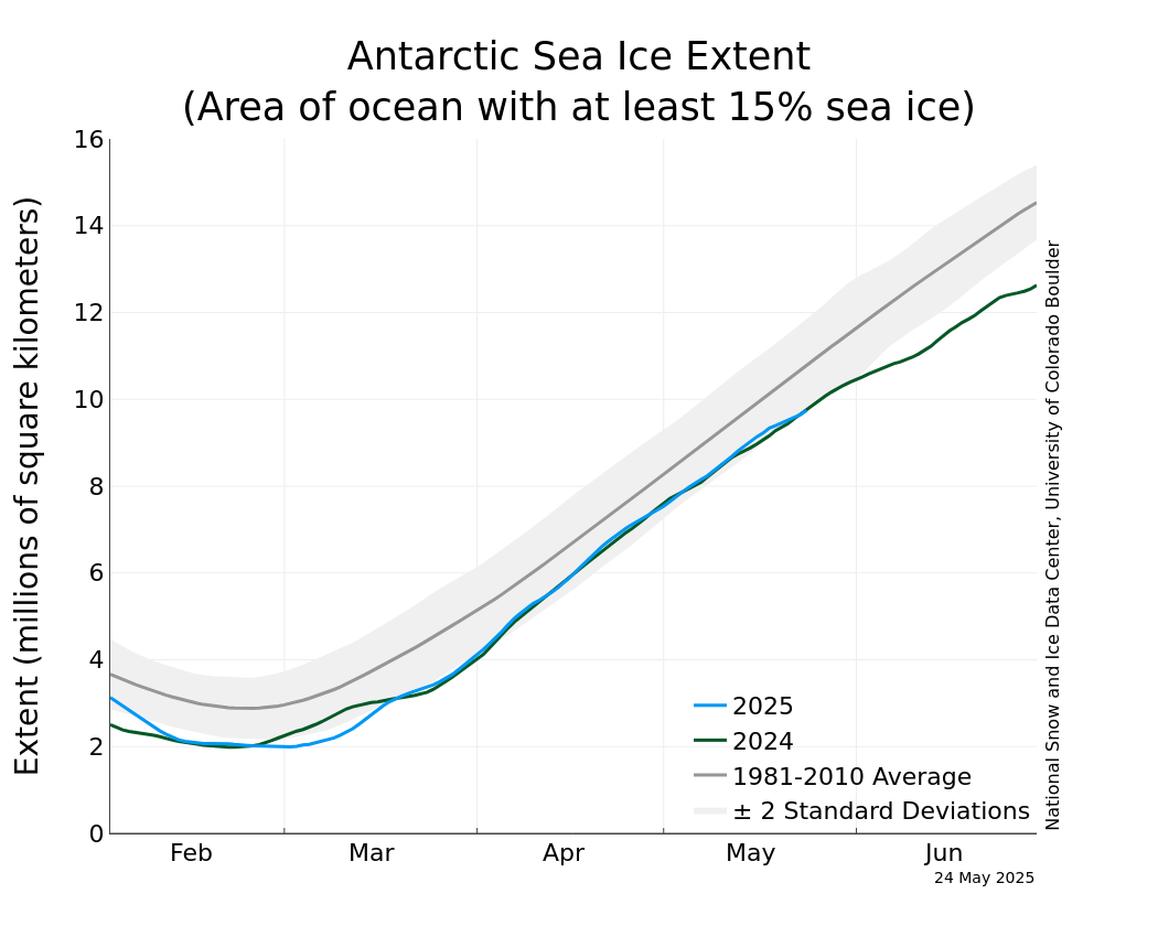
Finally, here is the Antarctic sea ice extent time series through early July:
The 2013 time series continues to track near the top of the +2 standard deviation envelope and above the 2012 time series. Unlike the Arctic, there is no clear trend toward higher or lower sea ice extent conditions in the Antarctic Ocean.
Policy
Given the lack of climate policy development at a national or international level to date, Arctic conditions will likely continue to deteriorate for the foreseeable future. This is especially true when you consider that climate effects today are largely due to greenhouse gas concentrations from 30 years ago. It takes a long time for the additional radiative forcing to make its way through the climate system. The Arctic Ocean will soak up additional energy (heat) from the Sun due to lack of reflective sea ice each summer. Additional energy in the climate system creates cascading and nonlinear effects throughout the system. For instance, excess energy pushes the Arctic Oscillation to a more negative phase, which allows anomalously cold air to pour south over Northern Hemisphere land masses while warm air moves over the Arctic during the winter. This in turn impacts weather patterns throughout the year across the mid-latitudes and prevents rapid ice growth where we want it.
More worrisome for the long-term is the heat that impacts land-based ice. As glaciers and ice sheets melt, sea-level rise occurs. Beyond the increasing rate of sea-level rise due to thermal expansion (excess energy, see above), storms have more water to push onshore as they move along coastlines. We can continue to react to these developments as we’ve mostly done so far and allocate billions of dollars in relief funds because of all the human infrastructure lining our coasts. Or we can be proactive, minimize future global effects, and reduce societal costs. The choice remains ours.
Errata
Here are my State of Polar Sea Ice posts from June and May 2013. For further comparison, here is my State of Polar Sea Ice post from July 2012.


 The EPA fuel economy estimates are a government guarantee on what fuel economy each vehicle will deliver.


